Emergent Complexity
One of reality’s enduring mysteries is emergence: how the whole becomes more than the sum of its parts. Aristotle recognized this over two thousand years ago. The question has been studied ever since.
No one has explained how simple rules produce complex behaviors. Yet cells following neighbor counts drift together across a screen. Bodies following gravity lock into resonances lasting billions of years. We’ve cataloged emergent phenomena across every field, but the rules alone never account for what we observe.
What we haven’t had is a framework that explains why certain configurations persist while others fall apart. Natural Reality provides one. General Selection operating on causal impedance determines what lasts.
Two demonstrations follow: one where everything is visible, one where causation stays hidden. The same mechanics operate in every system you navigate.
Contents
10.1 Hidden Layers of Complexity
10.1.1 From Invisible to Self-Evident
10.2 Solving Conway’s Game of Life
10.2.1 Selection and Persistence
10.2.2 Contextual Impedance and Variability
10.2.3 The Dynamics of Resistance
10.2.4 How Impedance Effectively Changes Rules
10.2.5 Life of a Glider
10.3 Solving The Three-Body Problem
10.3.1 Modulation of Causal Impedance
10.3.2 Adaptive Gravitational Dynamics
10.4 Complexity Matters
10.5 Closing Remarks
10.1 Hidden Layers of Complexity
Formations often develop in ways that seem unrelated to the rules that create them. Simple instructions can produce behaviors that look intricate from the outside. The right perspective makes the underlying interactions visible.
Most approaches to complexity focus on what appears at the surface and try to make sense of it. The analysis reveals connections on the surface, but the conditions guiding persistence stay out of view. Complexity lives in the processes that decide what continues and what fades. The visible result is only the outcome.
Conway’s Game of Life gives a direct look at this. Its rules are short and clear, yet they generate a surprising range of behaviors: gliders, oscillators, stable forms, and entire regions that reorganize step after step. Watching these developments exposes how much happens inside a system that seems almost too simple to produce anything interesting.
In An Introduction to Conway’s Game of Life, a YouTube video by Eric Steinhardt, this feeling is captured live:
“There seems to be a distinctive layer of reality, a second layer of reality on top of space.” (Steinhardt, 2024)
When the glider begins to drift, he pauses and notes how unexpected it feels. Five cells blink in place, yet a formation moves across the grid. Each cell obeys the same local rule, but the arrangement acts as if it has a life of its own.
This reaction is common. When only the surface is visible, the forces driving persistence stay hidden. The behavior looks spontaneous even though every update is determined.
Many areas of complexity science meet this same limit. Whether studying interacting bodies, chaotic motion, or large-scale emergent behavior, the deeper influences stay concealed when examined only through their visible outcomes. The surprise comes from the difference between what we see and what moves the system forward.
10.1.1 From Invisible to Self-Evident
Complexity feels mysterious when you see only the surface. Natural Reality distinguishes two orthogonal domains: the Interpretative Domain, where meaning gets organized, and the Causation Domain, where interactions unfold. Causal impedances and selection pressures determine which configurations persist.
The glider in Conway’s Game of Life offers a clear analogy. Its motion arises entirely from geometry repeating the conditions that sustain it. Viewed in this way, the glider shows how stable behavior can express itself when only the surface is available. The reason the arrangement endures lies in local conditions, not in any hidden mechanism.
Interpretation presents a horizontal surface while the influences driving behavior operate in a vertical domain. Formations stabilize, reorganize, or fade away according to how interactions accumulate across the system.
Natural Reality shows these dynamics. General Selection determines what persists. Causal impedance determines how transitions contribute to stability. When these harmonize, things endure. When they diverge, reorganization follows.
Once both contexts are recognized, complexity becomes clearer. The surface remains the same, yet the underlying dynamics become accessible. What once seemed puzzling settles into view.
10.2 Solving Conway’s Game of Life
The Game of Life is a cellular automaton played on an infinite grid where each cell is either alive or dead. At every step, the state of each cell is determined by simple, local rules:
- Birth: a dead cell becomes alive if exactly three of its neighboring cells are alive.
- Survival: a living cell remains alive if it has two or three living neighbors.
- Death: a living cell dies if it has fewer than two neighbors (isolation) or more than three neighbors (overcrowding).
Each cell in Conway’s Game of Life acts as an independent process, applying the same local rules to decide its next state based on its surroundings.
Here we take up a different puzzle: why motion and stability feel mysterious when you look only at local updates, and how Natural Reality gives a precise way to read that behavior.
A Life cell has no inner world; it isn’t a natural process. Its only happening is the change from one state to another. That simplicity makes it useful. Everything it does is fully exposed, and everything we take from it comes from how we read its behavior. This gives us a clear view of how formations propagate in a toy universe built from only local rules and visible outcomes.
We use Natural Reality here as a way to read what the geometry is doing. The automaton itself contains no interpretative domain and no causal impedances. Everything comes from the arrangement of cells. Geometry determines which rules activate, and persistence requires those local rule activations to rebuild a geometry capable of triggering the same balance again. Natural Reality gives us language for that balance. It lets us describe why certain transitions support what continues and others dissolve it. In a universe with no hidden states, stability comes entirely from geometry repeating the conditions that sustain it.
Although the Game of Life has no Interpretative or Causation Domains, it still exhibits a limited form of selection. The rules filter which geometries can recreate themselves and which collapse. This is a form of rule-compatibility selection: the automaton keeps only the arrangements that its own rules can rebuild. We use the language of Natural Reality to read this behavior because it reveals why some geometries persist and others dissolve, even though the system contains none of the machinery of natural processes.
In natural systems, Natural Reality describes General Selection operating on causal impedance. The Game of Life has neither: it’s a system with no Causation Domain and no internal states. We use Natural Reality’s language here as an interpretative framework, reading the automaton’s behavior through what we’ll call contextual impedance: how readily the rules reconstruct a geometry based on its configuration and context. When we say selection in this chapter’s Game of Life sections, we mean the contextual filtering the rules perform. When we say impedance, we mean contextual impedance unless we specify causal impedance.
Stable formations persist because their contextual impedances harmonize in ways that prevent disruptive transitions.
The rules of the Game of Life create interactions that produce what we see. These adapt, developing stable configurations that balance change and constraint. What we usually refer to as coherence is, in Natural Reality, harmonized Incoherence: variation and stability in a relationship that allows persistence without rigid uniformity.
How do stable, organized behaviors develop from a system governed solely by local, deterministic rules? Why do some formations survive while others vanish? What determines whether a formation persists, propagates, or disappears?
10.2.1 Selection and Persistence
Every change in the Game of Life is dictated by local conditions, yet larger formations exhibit behaviors that seem autonomous. Gliders traverse the grid, oscillators repeat in cycles, and some patterns trigger cascading transformations. The underlying rules produce these configurations and govern how influence flows through the system.
Many formations disappear immediately, while others persist indefinitely.
Different types show the principle:
- Still Lifes: completely stable configurations that never change (e.g., the 2×2 block).
- Oscillators: configurations that repeat in cycles (e.g., the Blinker).
- Gliders: moving configurations that propagate across the grid.
- Chaotic Regions: areas where cells constantly transition, failing to stabilize into anything persistent.
Contextual selection alone doesn’t fully explain how processes interact. Another factor determines how influence moves across processes and whether formations persist despite environmental fluctuations: contextual impedance.
10.2.2 Contextual Impedance and Variability
Contextual selection determines which formations persist. Contextual impedance governs how changes propagate within the system, structuring interactions and regulating whether transitions reinforce stability or drive reorganization.
State transitions don’t all happen with equal ease. The same rule applies differently depending on local conditions.
10.2.3 The Dynamics of Resistance
In Natural Reality, we read each cell’s transitions through impedance values that determine how rule effects express themselves based on local conditions. Every cell follows the same fundamental rules, but their effects vary with geometric context.
Formations endure when their impedances harmonize. A 2×2 block survives because impedance values in its cells harmonize across birth and death transitions.
Gliders persist through different mechanics. Transitions in a glider harmonize across cells in ways that produce coordinated motion. Impedances change as the formation moves, maintaining harmony while changing position.
Chaotic regions fail to form persistent configurations because impedances don’t harmonize. Cells transition rapidly as these values conflict rather than coordinate. No stable configuration develops because they never align.
10.2.4 How Impedance Effectively Changes Rules
Each cell’s rule application produces effects we interpret through impedance patterns. The same rule leads to different outcomes depending on geometry. Impedance describes how rules produce different effects, capturing variability in how the same conditions play out.
Formations survive when impedance patterns harmonize across cells. Different formation types show different harmonization results.
- Still Lifes remain completely stable. Impedances across all three rules (birth, survival, death) harmonize perfectly between neighbors. The 2×2 block maintains this harmony indefinitely.
- Oscillators harmonize in cycles. The Blinker alternates between two states because impedances harmonize at each phase of the cycle.
- Gliders harmonize while shifting position. Each step maintains harmony through a different configuration, creating coordinated motion across the grid.
- Chaotic Regions fail to harmonize. Transitions cascade without settling into stable conditions, preventing any persistent configuration from taking hold.
Contextual impedance captures how variability expresses itself within the system. These dynamics interact with contextual selection pressure, reinforcing what persists while dissolving what fails to sustain harmonization.
Contextual impedance as an interpretative framework bridges deterministic rules and emergent behaviors. Without it, we couldn’t explain why some configurations persist while others dissolve under identical rules. Variability in contextual impedance shows how contextual selection operates dynamically, reinforcing stable configurations while destabilizing Incoherent ones.
The Game of Life shows how contextual selection and contextual impedance guide emergent complexity. The same principles appear in physical systems, where motion and stability follow underlying constraints. The Three-Body Problem shows how deterministic interactions operate through organized constraints, producing motions that remain fully governed yet difficult to anticipate from a limited perspective.
10.2.5 Life of a Glider
Interpretation guides how we read what happens in the Game of Life. The automaton exposes every update directly, and Natural Reality lets us see why some arrangements keep going while others fade. The glider gives a clear case where repeated local conditions support steady motion.
Consider a glider starting at this configuration:
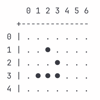
Five living cells form the characteristic glider shape. Over four iterations, this recreates itself one cell down and one cell to the right, drifting diagonally across the grid. Each cell stays fixed in its grid position, simply applying its internal rules based on local context. The glider survives because its geometry creates conditions that transform small variations into stable, coordinated motion.
Conway’s Game of Life is not a natural process. It has no causal impedance, no stored history, and no General Selection built into its rules, only the contextual selection we read from outside. A Life cell has no inner world. Nothing actually moves, nothing stores memory, repetition looks like motion.
We use Natural Reality as an interpretative tool here, reading how stability and variation behave inside the automaton. The impedance values below are not properties of the automaton. They are metrics we impose from outside to read why some transitions support a formation’s persistence while others cause it to dissolve. In natural processes, causal impedance operates: a process genuinely resists or accepts change based on internal conditions. In Life, contextual impedance is interpretative: a way to measure pattern stability.
In Life, impedance is interpretative: a way to measure pattern stability. But nothing pushes or resists change beyond the rules themselves. When we talk about lower or higher impedance, we’re not adding a new force to the grid; we’re describing how readily the existing rules reconstruct a geometry that can repeat itself.
The glider persists because its geometry creates repeating neighbor conditions that recreate itself one step over. We read this persistence through impedance harmonization: low impedance transitions (like trailing edge deaths around Z_d = 0.85) balance high impedance transitions (like center survivals around Z_s = 1.13). Random configurations with similar geometries dissolve because their transitions don’t coordinate this way. The impedance framework lets us identify what distinguishes persistent configurations from dissolving ones, even in a universe with no actual impedance mechanisms.
The walkthrough below uses impedance values to read the glider’s persistence. Each cell operates as a process containing three rules. Birth activates when dead with 3 neighbors. Survival activates when alive with 2 to 3 neighbors. Death activates when alive with fewer than 2 or more than 3 neighbors. The cell evaluates its neighbor count, determines which rule applies, and executes that rule.
Each rule expresses its own form of impedance. A cell doesn’t carry a single resistance value. When birth activates, we read one impedance (Z_b). When survival activates, we read another (Z_s). When death activates, we read yet another (Z_d). These values reflect how strongly a transition contributes to stability. Higher impedance values mark transitions that strain harmonization. Lower values mark transitions that reinforce it.
The isolated cell at (1,2) sits alive with only one neighbor at (2,3). The death rule activates with low impedance (Z_d = 0.88). The cell dies cleanly, removing an isolated component before it can destabilize the formation.
The dead cell at (2,1) counts three living neighbors at (3,1), (3,2), and (2,2). The birth rule activates. This transition reflects very low impedance to birth (Z_b = 0.92). The cell births, establishing a new leading edge for the formation. Contextual selection operates here: transitions that reinforce the formation’s integrity are the ones that persist.
The center cell at (3,2) has three neighbors and sits alive. The survival rule activates. We read this as taking place under slightly elevated impedance to survival (Z_s = 1.08). The cell stays alive. This variation could destabilize a less harmonized pattern. In the glider, the geometry expresses an impedance balance that absorbs it. The surrounding cells compensate, keeping the formation harmonized.
Cell (2,3) sits alive with two neighbors. The survival rule activates with moderate impedance (Z_s = 1.02). Cell (3,1) sits alive with two neighbors, activating the survival rule with low impedance (Z_s = 0.96). Cell (3,3) sits alive with three neighbors, activating the survival rule with slightly elevated impedance (Z_s = 1.11). The variation matters. A random configuration facing impedances ranging from Z_s = 0.96 to Z_s = 1.11 across survival transitions would fragment. The glider persists because we can read these variations as harmonizing. Low impedance in one survival balances higher impedance in another. The collective arrangement channels variation into coordinated change rather than chaos.
After one iteration:
The glider moved downward. Cell (1,2) died with Z_d = 0.88, clearing space. Cell (2,1) birthed with Z_b = 0.92, extending forward. Cell (4,2) birthed with Z_b = 0.98, supporting the bottom edge. Cell (2,3) survived with Z_s = 1.02, maintaining position. These transitions happened independently, yet we can read their impedances as harmonizing such that each cell’s rule application moved the glider collectively. Contextual selection favors configurations whose impedances harmonize across updates.
Cell (2,1) now has only one neighbor and sits alive. The death rule activates with low impedance (Z_d = 0.87). The cell dies, removing what became an isolated position. This transition fits what persists under contextual selection.
Dead cell (3,1) counts exactly three neighbors at (2,2), (3,2), and (4,2). The birth rule activates with low impedance (Z_b = 0.94), extending the leading edge again.
Cell (2,3) has two neighbors and sits alive. The survival rule activates. Natural Reality reads this as taking place under slightly elevated impedance (Z_s = 1.05). The cell stays alive. This survival maintains the upper boundary, necessary for the diagonal drift to continue.
Cell (3,3) has two neighbors and sits alive. The survival rule activates in a near-standard context (Z_s = 0.99).
Dead cell (4,3) has three neighbors at (3,3), (4,2), and (3,2). The birth rule activates with elevated impedance (Z_b = 1.08). The cell births, and the variation gets absorbed into the formation’s arrangement.
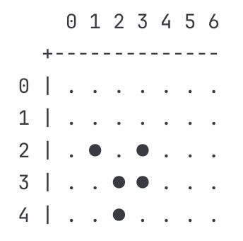
After two iterations:

The glider moved right and down. Cell (2,1) died with Z_d = 0.87 while cell (3,1) birthed with Z_b = 0.94 and cell (4,3) birthed with Z_b = 1.08. The birth at (4,3) occurred at high impedance (Z_b = 1.08), creating an inflection point where this could have fragmented. A random configuration would amplify this variation, but the glider absorbs it. Cell (3,2) survived with Z_s = 1.03, providing stability that allowed the higher-impedance birth at (4,3) to complete without destabilizing the whole. We can read the persistence as the result of harmonized impedance across different rule types. Birth impedances, survival impedances, and death impedances coordinate rather than conflict.
The isolated cell at (2,2) has one neighbor and sits alive. The death rule activates. This transition expresses very low impedance (Z_d = 0.85). The cell dies, clearing the formation’s trailing edge.
Dead cell (3,2) faces three neighbors at (2,3), (3,3), and (4,2). The birth rule activates with near-standard impedance (Z_b = 0.96), establishing the new center position.
Cell (3,3) has three neighbors and sits alive. The survival rule activates. Natural Reality reads this as the highest impedance we’ve seen (Z_s = 1.13). The cell stays alive. This context strains harmonization. In a random pattern, this kind of variation would propagate, amplifying until the formation dissolved. The glider absorbs it.
Cell (4,2) has three neighbors and sits alive. The survival rule activates in a low-impedance context (Z_s = 0.98), stabilizing the bottom edge.
Dead cell (4,4) sits with three neighbors at (3,3), (4,3), and (3,4). The birth rule activates with moderate impedance (Z_b = 1.02), easy to absorb.
After three iterations:
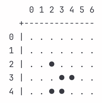
The glider continues its diagonal drift. Cell (2,2) died with Z_d = 0.85, removing trailing material. Cell (3,2) birthed with Z_b = 0.96, extending the center. Cell (4,4) birthed with Z_b = 1.02. Cell (3,3) survived with Z_s = 1.13. That survival was the critical inflection point. If impedances hadn’t harmonized across rule types, that high-impedance survival would have broken things. Instead, the low-impedance death (Z_d = 0.85) and the near-standard birth (Z_b = 0.96) compensated. We can read this as maintaining itself via coordinated change where impedance variations balanced across births, deaths, and survivals rather than amplifying.
Cell (2,3) has one neighbor and sits alive. The death rule activates in a low-impedance context (Z_d = 0.89), dying cleanly.
Dead cell (3,3) has three neighbors. The birth rule activates. This reflects very low impedance (Z_b = 0.87), establishing the new leading position.
Dead cell (4,4) sits with three neighbors at (3,4), (4,3), and (5,3). The birth rule activates with elevated impedance (Z_b = 1.05), consistent with the geometry.
After four iterations:

The glider restored its original pattern, moved one cell down and one cell right. Four iterations completed one full cycle. The pattern at (2,3), (3,4), (4,2), (4,3), (4,4) mirrors the initial configuration at (1,2), (2,3), (3,1), (3,2), (3,3), translated diagonally.
The glider’s motion comes from impedance harmonization operating under selection pressure across multiple rule types. At each iteration, cells apply whichever rules their local contexts activate: birth, survival, or death. Each rule expresses its own impedance, creating real variation and moments where this could fragment.
This gives us the simplest possible setting for seeing how contextual selection treats different configurations. Things persist when their impedances across all transition types transform variation into coordinated behavior. Things dissolve when variations amplify across transition types into disorder. The glider survives because its geometry generates conditions that Natural Reality identifies with stability.
When cell A births with Z_b = 0.92, it changes the neighbor count for cell B. If B’s survival rule activates with Z_s = 1.13, that elevated impedance could break coordination. The glider persists because cell C’s survival activates with Z_s = 0.96, compensating for B’s context. It continues because impedance variations balance across the whole configuration.
Random configurations dissolve because their impedances conflict across rule types. One cell’s birth at Z_b = 0.7 causes exaggerated extension. A neighboring cell’s survival at Z_s = 1.4 barely maintains position. Another cell’s death at Z_d = 1.3 fails to clear unstable material. The mismatches amplify. Within a few iterations, this fragments because the geometry creates contexts that fight rather than balance.
The glider avoids this fate via geometry that generates harmonized impedances across all three rule types. The five-cell arrangement creates neighbor configurations that activate rules in sequence. Birth impedances stay in ranges where extensions support what continues. Death impedances stay in ranges where removals clean trailing edges. Survival impedances stay in ranges where maintenance preserves geometry. The variations balance. Births with Z_b = 0.92 compensate for survivals with Z_s = 1.13. Deaths with Z_d = 0.87 clear material that would otherwise accumulate. This channels variation across multiple transition types into stability rather than chaos.
The glider’s motion looks like this:
Its motion comes from local rule applications that we can read as harmonizing across the arrangement. Birth impedances, survival impedances, and death impedances absorb variation together, recreating itself one position over via four iterations of synchronized transitions across multiple rule types.
Each cell simply applies its rules based on neighbor count and state. The survival of this particular configuration over countless others comes from selection pressure favoring configurations where impedances harmonize across all three rule types. That harmonization is what gets selected, why the glider persists while random configurations vanish.
The same logic applies when we move from this toy universe to neurons, markets, or planetary systems. The glider shows how a simple rule-based universe expresses configurations that persist when variation gets absorbed into stable conditions across multiple transition types. It gives a stripped-down example of the organizing principle that appears in natural complexity.
The Game of Life showed how selection and impedance operate in a toy universe built from simple rules. Every transition was visible, every geometry fully exposed. The blindfold didn’t operate there because the automaton has no internal states and no Red Space. Everything it does sits in plain view.
Now we move into natural systems where the blindfold returns in full force.
Natural processes have internal states we can’t observe, operating through causation we also can’t see. The three-body problem operates through General Selection and causal impedance: no longer the contextual versions we used to read the automaton, but the mechanisms that govern natural complexity.
10.3 Solving The Three-Body Problem
A single body drifts through space in a straight path. Two bodies orbit each other in predictable ellipses. Newton solved this centuries ago. Add a third body and the math stops working. No general solution exists for three bodies influencing each other gravitationally.
The equations fall short because of perspective. We model the system from our viewpoint, projecting our interpretations onto processes that each operate from their own position, velocity, and momentum. The blindfold hides this completely. We see three objects in space and calculate their trajectories from outside, missing that each body responds to gravity from its own internal model.
Jupiter doesn’t experience its own gravity the same way its moons do. Each moon responds to Jupiter, the Sun, and other moons from its own velocity and position. Our equations treat these as external variables we can measure from outside. But each body operates from inside its own frame, responding to forces in ways our external perspective can’t fully capture. We see three objects and calculate where they’ll be. Each object experiences gravitational influence from conditions we don’t observe directly. The mathematics fails at exactly the point where internal states matter most.
Stable configurations exist everywhere. Jupiter’s moons orbit in precise 4:2:1 resonance. The asteroid belt contains distinct gaps where gravitational interactions with Jupiter prevent stable orbits. Planetary systems settle into configurations that persist for billions of years.
These configurations emerge through General Selection operating on harmonized causal impedances. Each body expresses causal impedance to gravitational influences based on its position, velocity, and alignment with other bodies.
A moon orbiting Jupiter expresses causal impedance to gravitational influences from Jupiter, the Sun, and other moons. When its position, velocity, and timing create causal impedances that harmonize with all three influences, its orbit remains stable. Change any of these factors and the causal impedances can fail to harmonize, destabilizing the orbit.
General Selection operates on these causal impedances. Harmonized configurations persist while conflicting ones dissolve. The system settles where impedances reinforce rather than disrupt each other.
10.3.1 Modulation of Causal Impedance
Causal impedance depends on three factors: distance, velocity, and alignment.
Distance controls how strongly one body’s gravity affects another. A moon close to Jupiter experiences different gravitational influences than a distant moon, expressing different causal impedances to Jupiter’s gravity based on this distance.
Velocity controls how quickly gravitational influences change a trajectory. A fast-moving body responds differently to gravitational pull than a slow-moving body at the same distance. The same gravitational influence produces different trajectory changes depending on velocity, affecting the causal impedance the body expresses.
Alignment creates periodic connections. When three bodies align repeatedly, their gravitational influences can harmonize. Jupiter’s moons Io, Europa, and Ganymede orbit in 4:2:1 resonance. For every four orbits Io completes, Europa completes two and Ganymede completes one. Every moment this alignment recurs, the gravitational influences reinforce their existing orbital conditions. The causal impedances harmonize in that synchrony.
10.3.2 Adaptive Gravitational Dynamics
Early planetary systems contain countless small bodies interacting gravitationally. Most configurations express causal impedances that don’t harmonize. Bodies collide, merge, or get ejected. The configurations that persist are those where causal impedances harmonize across multiple interacting bodies.
A planetesimal in an unstable orbit expresses causal impedances that accumulate rather than canceling out, amplifying disturbances until the body gets ejected or collides with something else.
In a stable orbit, a planetesimal expresses causal impedances that harmonize with surrounding gravitational influences. Perturbations from different bodies cancel out or reinforce the trajectory. These align, dampening disturbances.
Over the course of many interactions, conflicting causal impedances dissolve while harmonized ones persist. The result is organized planetary systems: planets in stable orbits, asteroid belts with gaps at resonant positions, moons in synchronized resonances.
Jupiter’s gravity creates gaps in the asteroid belt at specific distances where asteroids would orbit in simple ratios with Jupiter (3:1, 5:2, 2:1 resonances). These positions create causal impedances that fail to harmonize. Gravitational tugs from Jupiter occur at the same point in each orbit, accumulating rather than averaging out, amplifying perturbations. Asteroids at these distances eventually get ejected or moved to orbits where causal impedances harmonize better. The gaps persist because any asteroid wandering into these positions expresses causal impedance that conflicts with stable orbital dynamics.
The three-body problem has no general mathematical solution, yet General Selection still determines which configurations persist. Harmonized causal impedances across interacting bodies produce stable arrangements, while conflicting ones lead to destabilization and dispersal.
10.4 Complexity Matters
The Game of Life and orbiting bodies are demonstrations. The same mechanics operate everywhere.
Your phone connects through dozens of intermediary steps. Your food travels through supply chains spanning continents. Your job depends on economic relationships operating beyond your direct observation. The Causation Domain, where actual happenings occur, is highly indirect.
Your mind interprets everything through flat cause-and-effect maps: direct connections, simple stories. The flat maps work fine for immediate physical interactions. They break down completely for the systems you live in today.
You want an outcome. You take what seems like a direct action. Nothing happens the way you expected. You try harder with the same approach. The confusion compounds. The systems you’re working with operate through pathways your interpretations miss entirely. You’re navigating multidimensional complexity with two-dimensional maps.
Causation operates orthogonally to interpretation. The indirect processes producing outcomes in modern life run perpendicular to the flat maps you use to understand them. The simplified stories you create feel complete while operating on different mechanics.
Recognizing that complexity operates in a dimension perpendicular to interpretation changes how you engage with the world. You model the indirection deliberately. You work with the mechanisms of how things happen. You stop applying two-dimensional interpretations to multidimensional processes.
Everything is complex under close examination.
The urgency lies in understanding human systems specifically. The gap between how causation actually works and how we think it works creates most of the confusion and dysfunction we experience. The framework gives you tools for thinking about processes operating beyond direct observation.
10.5 Closing Remarks
For centuries, complexity was difficult to understand because the surface behaviors drew all the attention. Natural Reality distinguishes what we experience from what produces it. We experience the Interpretative Domain while the conditions that produce stability and change develop in the Causation Domain, orthogonal to interpretation.
Conway’s Game of Life shows how things endure when contextual impedances across local updates support one another. The three-body problem shows how gravitational systems settle into long-lived arrangements through the same principle, with trajectories holding steady when their interactions reinforce rather than strain one another.
General Selection works across both domains. Configurations with causal impedances that fit together continue. Configurations with conflicting causal impedances fall away. Neural networks, economic systems, and ecosystems follow this same dynamic of General Selection acting on causal impedance across many interacting processes.
Seen in this way, long-standing questions about motion, stability, and emergence become workable. Things last when causal impedances support persistence. Systems adapt or change when new conditions either integrate into that support or press against it.
Orthogonality makes this visible. Happening runs perpendicular to interpretation. Once both contexts are recognized, their interaction becomes something we can describe and work with rather than something that only feels confusing at the surface.
Part III formalized causality and described how complexity emerges from General Selection acting on causal impedance across interacting processes. Part IV turns to practice and explores what’s possible when we use this way of seeing to guide how we participate in reality.
